Observation models

An observation model $z_k = h(\mathbf{x_k}) + w_k$ expresses a sensor’s observations $z_k$ at time instances $t_k$ given the state vector $\mathbf{x}$ . $w_k$ is assumed to be white gaussian noise with covariance matrix that depends on the specific sensor. The selection of the state vector $\mathbf{x}$ can lead to linear or nonlinear observation models.

Radar

The radar observation model includes calculating the distance and bearing from the own-ship to the target in polar form $z_{radar} = \begin{bmatrix} \rho, \theta \end{bmatrix}^{T}$ , given the target’s position $\begin{bmatrix}x_t, y_t\end{bmatrix}^{T}$ w.r.t the sensor’s coordinate system..

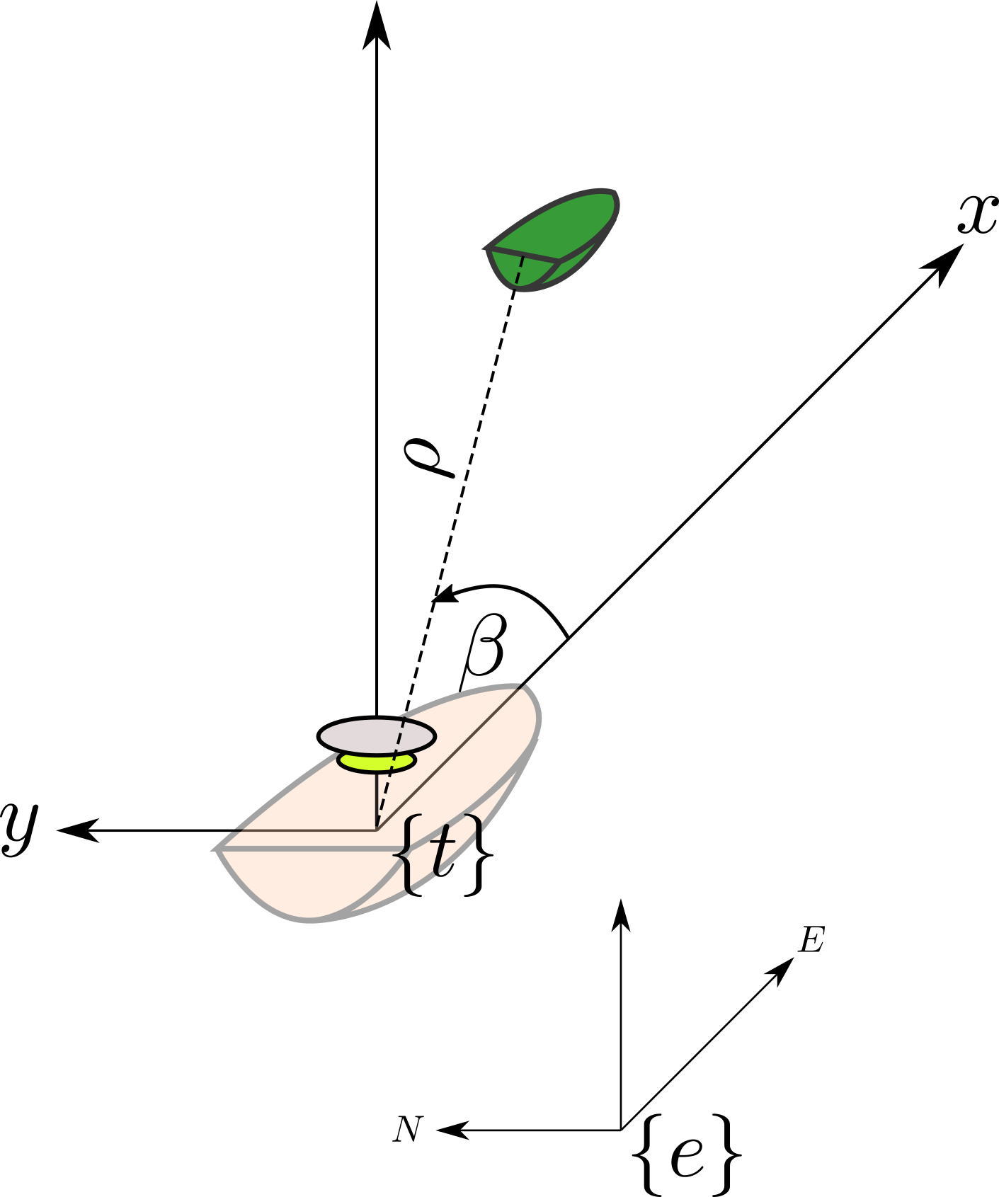
If the radar’s coordinate system, is for simplicity chosen to coincide with the tracking coordinate system, then the radar observation model can be expressed as:

$$ z_{radar}(\mathbf{x}) = \begin{bmatrix} \rho \\ \theta \end{bmatrix} = \begin{bmatrix} \sqrt{x^2 + y^2} \\ arctan(\frac{y}{x}) \end{bmatrix} + w_{radar} $$

where the observation noise $w$ is commonly assumed to be white, zero-mean Gaussian with covariance $R_{radar} = \text{diag}\left[\sigma^2_{\rho}, \sigma^2_{\theta}\right] $

A reasonable sizing of the noise variances can be

• $\sigma^2_\rho = 10 [\textit{m}]$
• $\sigma^2_\theta = 3 \frac{\pi}{180} [\textit{rad}] $

GPS

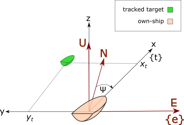
A GPS observation model calculates the target’s relative position $\begin{bmatrix}x, y\end{bmatrix}^{T} $ w.r.t the own-ship’s tracking coordinate system, which is directly a part of the state vector, given the target’s state vector $\mathbf{x}$

• The own-ship’s geodetic coordinates $\begin{bmatrix}\phi_{0}, \lambda_{0} \end{bmatrix}^{T}$
• The own-ships sea-keeping heading angle from true north $\psi_{\textit{0}}$
• The target’s measured geodetic coordinates $\begin{bmatrix}\phi, \lambda\end{bmatrix}^{T}$ which is usually available at sea through the Automatic Identification System.

$$ z_{GPS}(\mathbf{x},\begin{bmatrix}\phi_{0}, \lambda_{0}, \psi_{\textit{0}} \end{bmatrix}^{T}) = \begin{bmatrix} x \\\\ y \end{bmatrix}{GPS} = \begin{bmatrix} x \\\\ y \end{bmatrix} + w{GPS} $$

The fact that the geodetic coordinates origin and the heading angle of the own-ship is not included in the state-space representation leads to a linear observation model.

The observations are pre-converted into tracking coordinates, and the noise is added on the the post-converted observations.

The AIS observations $[\phi, \lambda]^{T}$ can be transformed into tracking coordinates $[x,y]^{T}$ by using the transformations from the relative chapter.

$$ \begin{bmatrix} x \\ y \end{bmatrix} = R_z(\frac{\pi}{2}-\psi_{\textit{0}}) \cdot F_1\left(F_2(\begin{bmatrix} \phi \\ \lambda \end{bmatrix}),\begin{bmatrix} \phi_0 \\ \lambda_0 \end{bmatrix}\right) $$

Where

• $F_2\left(\begin{bmatrix} \phi \\ \lambda \end{bmatrix}\right)$ is the transformation from geodetic to ECEF coordinates

• $F_1\left( \begin{bmatrix} X \\ Y \\ Z \end{bmatrix}_{ECEF},\begin{bmatrix} \phi_0 \\ \lambda_0 \end{bmatrix}\right)$ is the transformation from ECEF to ENU, given the geodetic coordinates of the own-ship $\begin{bmatrix} \phi_0, \lambda_0 \end{bmatrix}^T$ as a reference point.

• $R_z(\theta)$ is the transformation from ENU to sea-keeping/tracking coordinate system..

AIS

An alternative method to using the aforementioned GPS model is to leverage the fact that the tracked targets are in the viscinity of the own-ship, and thus small differences in geodetical coordinates can be linearly mapped to ENU differences and the other way around.

$$ \begin{bmatrix} \phi\\ \lambda \end{bmatrix}_{\text{target}}= \begin{bmatrix} \phi_{0}\\ \lambda_{0} \end{bmatrix}_{\text{own-ship}} + \begin{bmatrix} \delta\phi \\ \delta\lambda \end{bmatrix} + w_{\textit{AIS}}$$

x [src:“Wikipedia:Geographic coordinate conversion”]

By differentiating the model mentioned in the Coordinate systems section, one can confirm that for given own-ship geodetic coordinates $(\phi_0,\lambda_0, h_0)_{\textit{own-ship}}$

$$ \begin{bmatrix} dE\\dN\\dU \end{bmatrix}= \begin{bmatrix} (N(\phi_0)+h_0)\cos\phi_0 &0 &0\\ 0 &M(\phi_0) + h_0 &0\\ 0 &0 &1 \end{bmatrix} \begin{bmatrix} d\lambda\\d\phi\\dh \end{bmatrix} $$

Tracking is performed at sea level, thus $h=0$, leading to

$$ \begin{bmatrix} d\lambda\\ d\phi \end{bmatrix}= \mathbf{T}(\phi)^{-1} \begin{bmatrix} dE\\ dN \end{bmatrix} $$

Since the target’s state is in the tracking/seakeeping coordinate system, one needs to transform it to ENU.

If $\mathbf{R}_z(\psi)$ is the Euler’s angle transformation for a rotation $\psi$ around the z-axis, then the transformation from sea-keeping/tracking to ENU

$$\mathbf{R}^{\textit{ENU}}_{\textit{sea-keeping}} $$

given the own-ship’s heading from true-north $\psi_{\textit{0}}$ is ,

$$R_{\textit{sea-keeping}}^{\textit{ENU}} = R_{z}(\frac{\pi}{2}-\psi_{\textit{0}})$$

$$ \begin{bmatrix} dE\\ dN \end{bmatrix}= R_{\textit{sea-keeping}}^{\textit{ENU}} \begin{bmatrix} x\\ y \end{bmatrix}_{\textit{{t}}} $$

and thus, by combining the above equations, one can solve for the observed $[\phi, \lambda]^{T}$,

$$ \begin{bmatrix} \phi\\ \lambda \end{bmatrix}= \begin{bmatrix} \phi_{0}\\ \lambda_{0} \end{bmatrix} + {\mathbf{T}(\phi_{0})}^{-1}\begin{bmatrix} dE\\ dN \end{bmatrix} + w_{\textit{AIS}}=$$

$$ \begin{bmatrix} \phi_{0}\\ \lambda_{0} \end{bmatrix}{\textit{own-ship}} + \mathbf{T}(\phi{0})^{-1} \mathbf{R}^{\textit{ENU}}{\textit{sea-keeping}}(\psi{\textit{0}}) \begin{bmatrix} X_{\textit{target}}\\ Y_{\textit{target}} \end{bmatrix}{\textit{wrt}{{\textit{sea-keeping}}}}+w_{\textit{AIS}} $$

Where

• $\mathbf{T}(\phi)= \begin{bmatrix} N(\phi)\cos\phi &0\\ 0 &M(\phi) \end{bmatrix} $ is the transformation matrix from geodetic differences to ENU differences.

• $N(\phi) = \frac{\alpha}{\sqrt{1-e^2\sin^2\phi}}$ is the prime vertical radius of curvature

• $M(\phi) = \frac{\alpha(1-e^2)}{(1-e^2\sin^2\phi)^\frac{3}{2}}$ is the meridional radius of curvature

• $\alpha,\beta$ are the equitorial radius(6378.1370 km) and the Polar radius(6356.7523 km) respectively, as derived from the WGS-84 ellipsoid model.

• $e = \sqrt{1 -\frac{b^2}{a^2}}$ is the ellipsoid’s eccentricity.

• $h = 0 $ since the own-ship is always floating on the geoid.

• $w_{\textit{AIS}}$ is white gaussian zero-mean noise with covariance matrix $\mathbf{R}_{\textit{AIS}}$ depending on the noise intensity of the AIS source.

The above equation can be rewritten to the standard observation model formulation

$$ z_{AIS}(\mathbf{x},\begin{bmatrix}\phi_{0}, \lambda_{0}, \psi_{\textit{0}} \end{bmatrix}^{T}) = \begin{bmatrix} \phi\\ \lambda \end{bmatrix}{\textit{target}} = \begin{bmatrix} \phi{0}\\ \lambda_{0} \end{bmatrix} + \mathbf{H}\mathbf{x} + w_{\textit{AIS}} $$

, which is a linear observation model that is approximating the geoid with a spherical-linearization about the own-ship’s geodetic location.

Camera

Assuming a camera sensor on a mast with the camera z-axis aligned with the own-ship’s body coordinate system

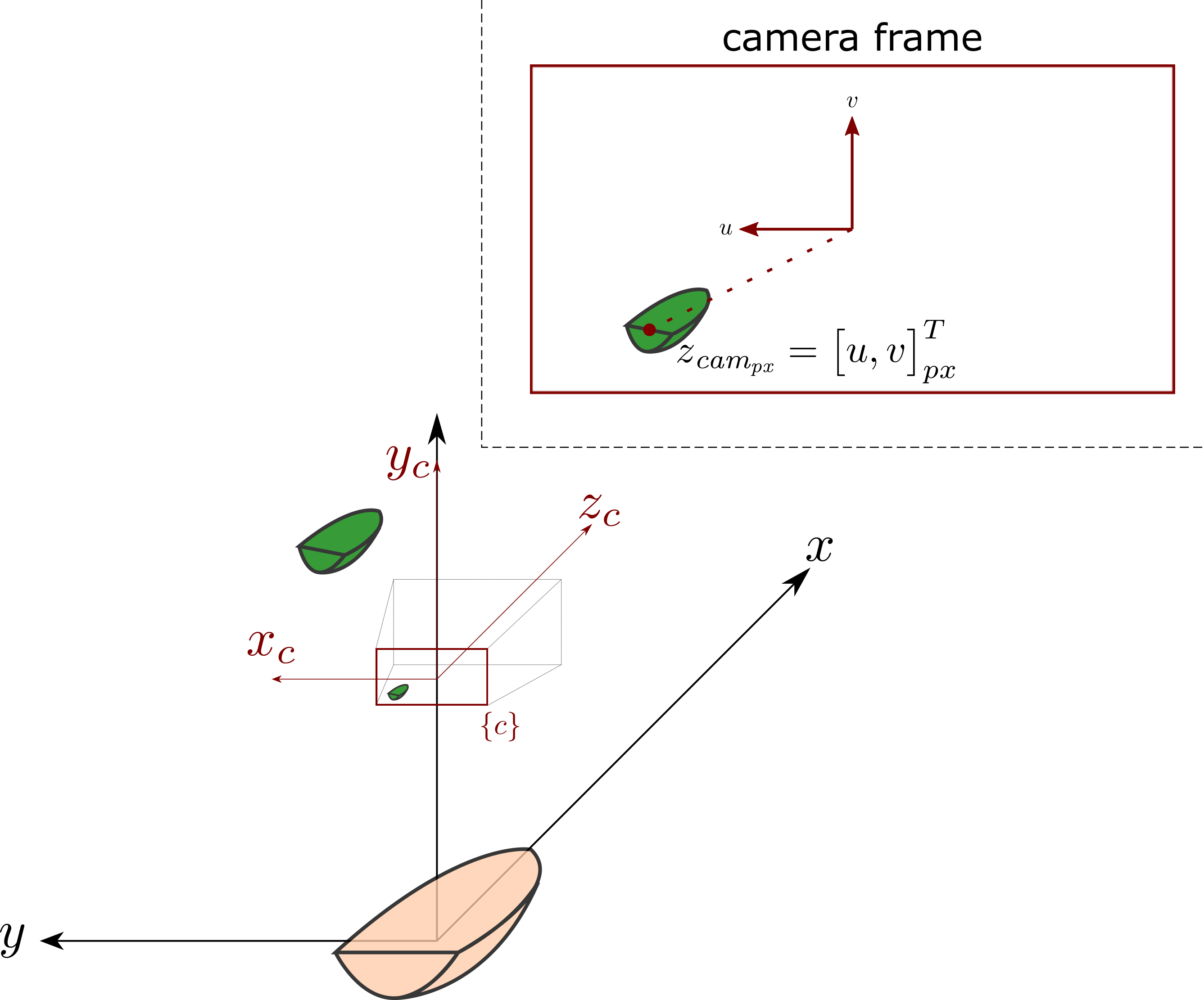
A top-view of the pinhole model seen in the figure below

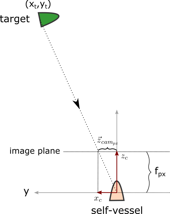
Then the observation model for the predicted pixel location of a target obtained from a deep neural-network classifier and localiser is found by projecting a point in homogeneous coordinates

$$x_{\text{wrt}_{\text{sea keeping}}} =\begin{bmatrix}x, y, 0, 1\end{bmatrix}^T$$

to the finite camera frame, given measured information $z_{gyro}$ about the rotational angle of the own-ship body coord system, w.r.t the tracking coord system

$$ z_{\textit{cam}{\textit{px}}}(\mathbf{x},z{\textit{gyro}}) = \begin{bmatrix}u\\v\end{bmatrix}{px}= \frac{\begin{bmatrix}-P_1-\\-P_2-\end{bmatrix}\mathbf{x}}{ \begin{bmatrix} -P_3- \end{bmatrix} \mathbf{x}}+ w{\text{camera}} $$

Where $\mathbf{P}$ is the projection matrix and $P_{i}$ it’s rows

$$ P = \begin{bmatrix}-P_1- \\-P_2-\\-P_3- \end{bmatrix} = \mathbf{K}\mathbf{R_{\textit{own-ship}}^{\textit{camera}}}[\mathbf{I} | \mathbf{-C}] \begin{bmatrix} \mathbf{\mathbf{R}_{\textit{sea-keeping}}^{\textit{own-ship}}} &\mathbf{0}\\ \mathbf{0} &1 \end{bmatrix}$$

Because of the denominator this is a non-linear model, and a description of the matrices that comprise the projection matrix $P$ is given below:

$\mathbf{K}$

is the intrinsic camera calibration matrix

$$\mathbf{K} = \begin{bmatrix}f m_x &0 &p_x \\ 0 &f m_y &p_y \\ 0 &0 &z \end{bmatrix} $$

with

• $f$ is the intrinsic camera calibration parameter, focal length in mm
• $m_x, m_y$ are the camera’s sensor pixel density in $\frac{\text{number of pixels}}{mm}$ across the two different directions of the image plane.
• $p_x,p_y$ correspond to the position of the principal point of the image in pixel coordinates
• $w_{\textit{camera}}$ is white gaussian zero mean noise with variance related to the classifier accuracy, or any calibration errors in the extrinsic and intrinsic camera matrices.

$\mathbf{R}_{\textit{own-ship}}^{\textit{camera}}$

is the extrinsic camera rotation matrix that describes the orientation of the camera coordinate system. w.r.t. the own-ship.

$\mathbf{C}$

is the extrinsic origin of the camera coordinate system. w.r.t. the own-ship.

$\mathbf{R}_{\textit{tracking}}^{\textit{own-ship}}$

Is the transformation matrix that corresponds to the roll-pitch rotation of the own-ship’s body coordinate system. w.r.t the tracking coordinate system.. Please note that the order of the rotations matters.

$$ R_{\textit{tracking}}^{\textit{own-ship}}=\left( R_{\textit{pitch}} R_{\textit{roll}}\right)^T $$

Where $$R_{\textit{pitch}},R_{\textit{roll}}$$ are the standard rotation matrices for Euler’s angles $z_{\textit{gyro}}=(\alpha,\beta)^T = (\textit{roll},\textit{pitch})^T$.

$$ R_{\textit{roll}}= R_x(\alpha) = \begin{bmatrix} 1 &0 &0\\ 0 &\cos\alpha &-\sin \alpha\\ 0 &\sin \alpha &\cos \alpha \end{bmatrix} $$

and

$$ R_{\textit{pitch}}= R_y(\beta) = \begin{bmatrix} \cos\beta &0 &\sin \beta\\ 0 &1 &0\\ -\sin \beta &0 &\cos\beta \end{bmatrix} $$

A basic assumption at that point, is that the own-ship is able to measure the angles $(\alpha,\beta)$ of the own-ship body coordinate system. w.r.t the tracking coordinate system.. These angles are usually available on a ship by using one or multiple gyroscope sensors.