Particle filtering

Particle filters (PFs) belong to the category of sub-optimal filters. They represent probability densities with point mass densities (“particles”), and perform Sequential Monte Carlo (SMC) estimations. SMC ideas were historically introduced in statistics from the 1950s but the limited computational power available at the time constrained their use and development. As soon as faster computers were made available, the related research activity in the field increased, resulting in their improvement and adoption in numerous applications, namely tracking, localisation of agents, pattern recognition, fault-detection, and ADAS.

Monte carlo integration

The basis of SMC methods is Monte Carlo integration. If a multidimensional integral needs to be evaluated:

$$\mathbf{I} = \int \mathbf{g(x)} d\mathbf{x}$$

where

$$ \mathbf{x} \in \mathbf{R}^{n_{x}} $$

Then the Monte Carlo (MC) approach for numerical integration assumes a factorisation

$$\mathbf{g(x)} = \mathbf{f(x)} \cdot \pi(\mathbf{x}) $$

so as that $\pi(\mathbf{x})$ is interpreted as a probability density which is satisfying

$$ \begin{align} \pi(\mathbf{x}) \geq 0 \ \int \pi \mathbf{x} d \mathbf{x} = 1 \end{align} $$

If one can “draw” $N » 1$ samples ${x^i; i = 1,…,N}$ distributed according to $\pi (\mathbf{x})$ , then the integral estimate can be approximated with the sample mean:

$$ I = \int \mathbf{f}(\mathbf{x})\pi(\mathbf{x}) d\mathbf{x} = I_N \approx \frac{1}{N}\sum_{i=1}^{N} \mathbf{f}(\mathbf{x}^i) $$

Given that the samples $\mathbf{x}^i$ are independent, then $I_N$ is an unbiased estimator, and according to the law of large numbers it will almost surely converge to $I$.

Given that the variance of $\mathbf{f}(\mathbf{x})$, $\sigma^2$ is finite,

$$ \sigma^2 = \int (\mathbf{f}(\mathbf{x})- I)^2 \pi(\mathbf{x}) $$

then the central theorem holds and the estimation error converges to the distribution:

$$ \lim_{N\rightarrow \inf} \sqrt{N}(I_N - I) \sim \mathcal{N}(0, \sigma^2) $$

In the Bayesian context, $\pi(\mathbf{x})$ conveniently corresponds to the posterior belief density. What is not convenient though, is the fact that the posterior is usually multivariate, nonstandard and only known up to proportionality, thus distributed sampling is usually not available from it. A solution to this is the use of Importance Sampling.

Importance sampling

In order to generate samples directly from $\pi (\mathbf{x})$ and estimate $I$ using Monte Carlo integration, one can generate samples from a density $q(\mathbf{x})$, which is similar to $\pi(\mathbf{x})$. The pdf $q(\mathbf{x})$ is usually referred to as importance or proposal density.

Similarity between $\pi \text{ - } q $ is expressed as:

$$ \pi(\mathbf{x}) > 0 \rightarrow q(\mathbf{x})>0 , \text{for all } \mathbf{x} \in R^{n_x} $$

which means that $q(\mathbf{x})$ and $\pi(\mathbf{x})$ have the same support. The integral $I$ can be rewritten thus as:

$$ I = \int \mathbf{f}(\mathbf{x}) d\mathbf{x} = \int f(\mathbf{x}) \frac{\pi(\mathbf{x})}{q(\mathbf{x})}q(\mathbf{x}) d\mathbf{x} $$

Applying the MC sample mean:

$$ I_N = \frac{1}{N} \sum_{i=1}^{N} \mathbf{f}(\mathbf{x}^i) \tilde{w}(\mathbf{x}^i) $$

where the importance weights shape a probability mass function(PMF), and thus need to be normalised.

$$ w(\mathbf{x}^i) \frac{\tilde{w}(\mathbf{x}^i)}{\sum_{j=1}^N \tilde{w}(\mathbf{x}^j)} $$

Bayesian estimation

As already mentioned, in the Bayseian context, $\pi (\mathbf{x})$ is the posterior density. For selecting the proposal distribution $q(\mathbf{x})$ it makes sense to try to mantain a degree of similarity between the proposal and the posterior, so that the finite $N$ selected $\mathbf{x}^i$ samples fall into probable regions of the posterior, that is regions that contain information about the actual posterior distribution $p(\mathbf{x} | z_i)$.

Sequential importance Sampling (SIS)

[reference to 1.3 and conceptual filtering solution]

Intuitively, a recursive Bayesian nonlinear filter is a very suitable domain for applying MC integration. This sequential Monte Carlo approach is known with various names such as,

• boostrap Filtering
• condensation algorithm
• particle Filtering
• survival of the fittest

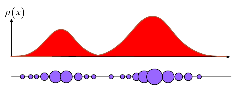
The key idea again, is to represent the posterior density function by a limited set of samples and their importance weights, based on which estimates can be calculated. As the number of samples increases, the sampled distribution becomes an equivalent representation to the functional description of the posterior pdf, and the SIS filter approaches the optimal Bayesian filtering estimator.

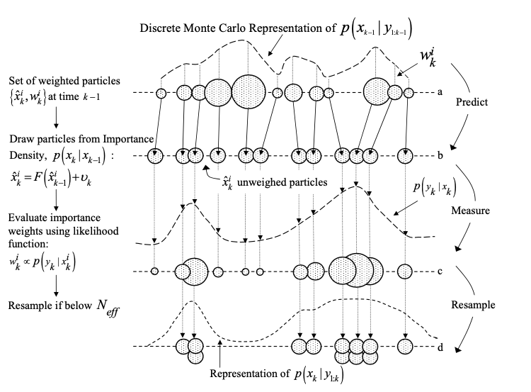
The recursive nature of SIS implies that the new weights describing the posterior $p(\mathbf{x}_k | \mathbf{z}_k)$ are being updated based on their previous values, and the likelihood of a new measurement $$p(\mathbf{z}_k | \mathbf{x}_k^i)$$, i.e

$$ w_k^i \sim w_{k-1}^i \frac{p(\mathbf{z}_k | \mathbf{x}_k^i)p(\mathbf{x}k^i | \mathbf{x}{k-1}^i)}{q(\mathbf{x}k^i | \mathbf{x}{k-1}^i , \mathbf{z}_k)} $$

Then the posterior filtered density is described as a pmf as:

$$p(\mathbf{x}_k | \mathbf{z}k) \approx \sum{i=1}^N w_k^i \delta(\mathbf{x}_k - \mathbf{x}_k^i)$$

The recursiveness of the algorithm is evident since the importance weights $w_k^i$ and support points $x_k^i$ are being propagated as each measurement is received sequentially. The SIS algorithm is the basis of most particle filtering algorithms, and the choice of the importance density function is crucial in the design.

Importance density selection

A popular and convenient selection of the importance density is the transitional prior, i.e. the motion model:

$$q(\mathbf{x_k | x_{k-1}^i , \mathbf{z}_k}) = p(\mathbf{x}k | \mathbf{x}{k-1}^i)$$

substituting the above in the SIS algorithm yields

$$ w_k^i \sim w_{k-1}^i p(\mathbf{z}_k | \mathbf{x}_k^i) $$

Degeneracy problem

A general problem of a SIS particle filter is that the particle distribution becomes extremely peaked through the subsequent measurement updates. That is, the variance of the importance weights can only increase over time. This effect overtime leads to poor accuracy of the estimates and leads to a common problem of the SIS particle filter, that of degeneracy. An effective countermeasure is monitoring the level of degenracy of the filter and resample when appropriate. Such a measure is the effective sample size $N_{\text{eff}}$ as introduced by ref]

$$ \hat{N}_{\text{eff}} = \frac{1}{\sum_{i=1}^{N}(w_k^i)^2} $$

One can easily verify that $$1 < N_{\text{eff}} < N$$ , thus a usual degeneracy criterion is

$$ \begin{aligned} N_{\text{eff}} &< \alpha N ,& \alpha \in \mathcal{R}: &\alpha \in (0,1) \end{aligned} $$

Resampling algorithms

Whenever a degeneracy is detected(i.e $N_{\text{eff}}$ falling below a threshold value), resampling is performed.

Resampling follows the strategy of survival of the fittest, by eliminating particles in the set with low weight values and replacing them with copies of the more probable ones.

The resampling algorithm is thus:

1. Normalize the particle set weights $w^j$
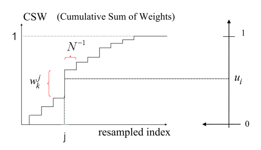
2. Calculate the Cumulative Sum of Weights(CSW) function $$F_k(i) = \sum_{j=1}^{i} w_k^j$$.
3. Draw $N$ random samples $u_i \in \mathcal{R}$, $i=1,..,N$ uniformly distributed on the interval $[0,1]$.
4. For every uniform sample $u_i$, pick $\hat{x}_k^i = x_k^j$ out of the current samples pool, where the picking index $j$ depends on the weight’s value as

$$ j = \underset{i}{\arg\min} |F_k(i)-u_i| $$

The above strategy leads to a weight selection survival chance equal to the weight’s value $P(\hat{x}_k^i = x_k^j) = w_k^j$ . This results in useful samples having a higher likelihood of being selected for the new set. The new weights of the samples are uniform i.e. the weights are set to

$$\{\hat{x}_k^i , 1/N\}$$

The use of resampling technique might lead to other issues though. Diversity among particles is depleted as highly probable particles are through subsequent resampling steps genetically dominating the distribution. Moreover, if the process noise is too low then the distribution will not diversify enough in between measurement updates and will eventually become a uniformly weighted replicate of a few particles. This phenomenon is also known as sample impoverishment or particle depletion . [ref].

PF Algorithm outline

The PF algorithm thus summarises to:

1. Initialise the filter by drawing particles according to an initial belief $p(\mathbf{x}_0)$

Usually $p(\mathbf{x}_0)$ is Gaussian with known moments, or a uniform distribution around the initial estimate $\mathbf{x}_{0}$.

2. Update the particle set weights according to a the likelihood of the new measurement.

   This step requires pointwise evaluation of the likelihood-function $p(\mathbf{z}_k | \mathbf{x}_k)$ which depends on the stochastic properties, of the measurement model.

   Example: For the radar sensor, the likelihood function is the multivariate gaussian: $$ p(z|x) = (2\pi)^{-\frac{k}{2}}\det{}(\mathbf{R})e^{-\frac{1}{2}\left(z-h(x))^{T}\mathbf{R}(z-h(x)\right)} $$ Where $\mathbf{R}_{k\times k}$ is the measurement noise covariance matrix

3. Normalise weights to represent a pmf.

4. Resample if required, based on $N_{\text{eff}} < \textit{threshold}$

5. Propagate every point according to the motion model.

   It is crucial to use non-zero process noise at that step, as that ensures that additional diversity is being introduced into the distribution.

6. Repeat from step #2

[ref]