Motion models

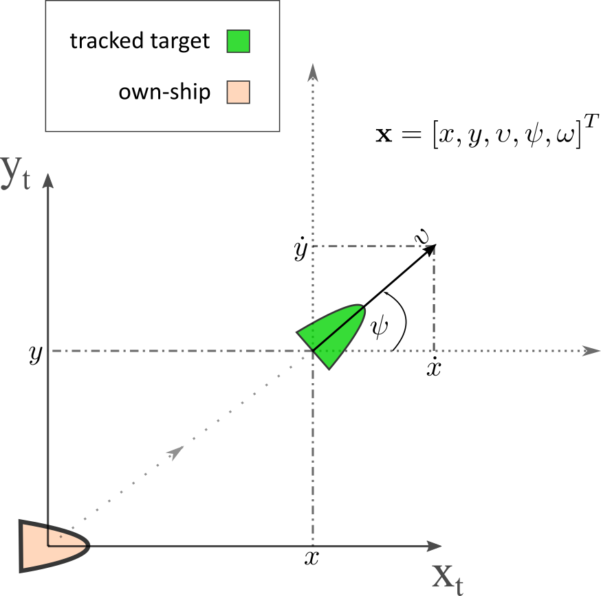
When choosing a coordinate system for the target motion model, it is very convenient to assume the target’s state on a the own-ship’s two dimensional tracking plane.

In order to improve the quality the stability and the accuracy of the estimations, the ships are assumed to comply with dynamic motion models. The tracking problem therefore is that of estimating the model’s parameters for a target, taking into consideration all available observations from various sensors.

The motion models proposed in literature are numerous. Trying to keep the complexity low, linear motion models assume a constant velocity(CV) or constant acceleration (CA). These models have the advantage that the state transition equation is linear, and thus the state distribution can be optimally propagated. Unfortunately they are limited to straight motions and are thus unable to capture rotations. If one introduces the angular speed of the target around its z-axis as well, the resulting models are referred to as curvilinear models.

Tracking coordinates

Tracking objects in the two dimensional equilibrium tracking frame is a fair assumption at sea since all targets in the vicinity of the own-ship are floating, and thus assuming their motion on a plane is a fair approximation as long as the distance between the tracked target and the own-ship is not large enough for the earth’s curvature to induce approximation errors. The model’s fidelity using the tracking coordinates is a topic of debate. In the context of sensor fusion and local situational awareness, the on-board sensors used on a ship operate within a range limit that should — at least intuitively — ratify the tangential plane approximation.

When it comes to situational awareness in a more global context, i.e. tracking targets across the Atlantic, one could argue that there is no sense in applying sensor fusion since the targets are observable solely through GPS measurements.

Continuous constant turn rate and velocity (CTRV) model

Starting with a time continuous model

$$\begin{aligned}\dot{\mathbf{x}}(t) = f(\mathbf{x}(t)) + w(t) &&,\mathbf{x} = \left[x,y,\upsilon, \psi,\omega\right]^{T} \end{aligned}$$

then assuming that the linear velocity $\upsilon$ and the turn rate $\omega$ remain constant — which is a fair assumption for a moving vessel — then the non-linear dynamics are

$$f =\begin{bmatrix}\dot{x} \\ \dot{y} \\ \dot{\upsilon} \\ \dot{\psi} \\ \dot{\omega} \end{bmatrix}= \begin{bmatrix}\upsilon cos(\psi) \\ \upsilon sin(\psi) \\ 0 \\ \omega \\ 0 \end{bmatrix}$$

which is describing constant turn rate and velocity(CTRV)model since the derivatives of the linear and angular velocities are zero .

[src: Comparison and Evaluation of Advanced Motion Models for Vehicle Tracking]

Discretisation of the CTRV motion model

Since the system is simulated in discrete time, one can integrate the motion model within a sample time $T$ and obtain exactly:

[src:ODE integration]

$$\begin{aligned} \mathbf{x}(t+T) = \mathbf{x}(t) + \int_{t}^{t+T}(f(\mathbf{x}(\tau)+w(\tau) )d\tau &&\text{and}&& f(\mathbf{x(\tau)})= \begin{bmatrix}\upsilon cos(\psi) \\ \upsilon sin(\psi) \\ 0 \\ \omega \\ 0 \end{bmatrix}\\ \mathbf{x(\tau)} = \left[x,y,\upsilon, \psi,\omega\right]^{T} \end{aligned}$$

and hence , the discrete update model(ignoring the noise) is

$$ \mathbf{x}(t+T) = g\left(\mathbf{x}(t)\right) $$

therefore, the non linear discrete state transition function $g(\mathbf{x}(t)$ by direct integration, for $\mathbf{x}(t) =\left[x,y,\upsilon, \psi,\omega\right]^{T} $,

$$ g(\mathbf{x}(t)) = \mathbf{x}(t) + \begin{bmatrix} \frac{2\upsilon}{\omega}sin(\omega T)cos(\psi + \frac{\omega T}{2})\\ -\frac{2\upsilon}{\omega}sin(\omega T)cos(\psi + \frac{\omega T}{2})\\ 0 \\ \omega T \\ 0 \end{bmatrix} , \omega \neq 0 $$

or

$$ g(\mathbf{x}) = \mathbf{x} + \begin{bmatrix} \upsilon T cos(\psi)\\ \upsilon T sin(\psi)\\ 0 \\ 0 \\ 0 \end{bmatrix} , \omega = 0 $$