Kalman and extended Kalman filtering
Kalman filter
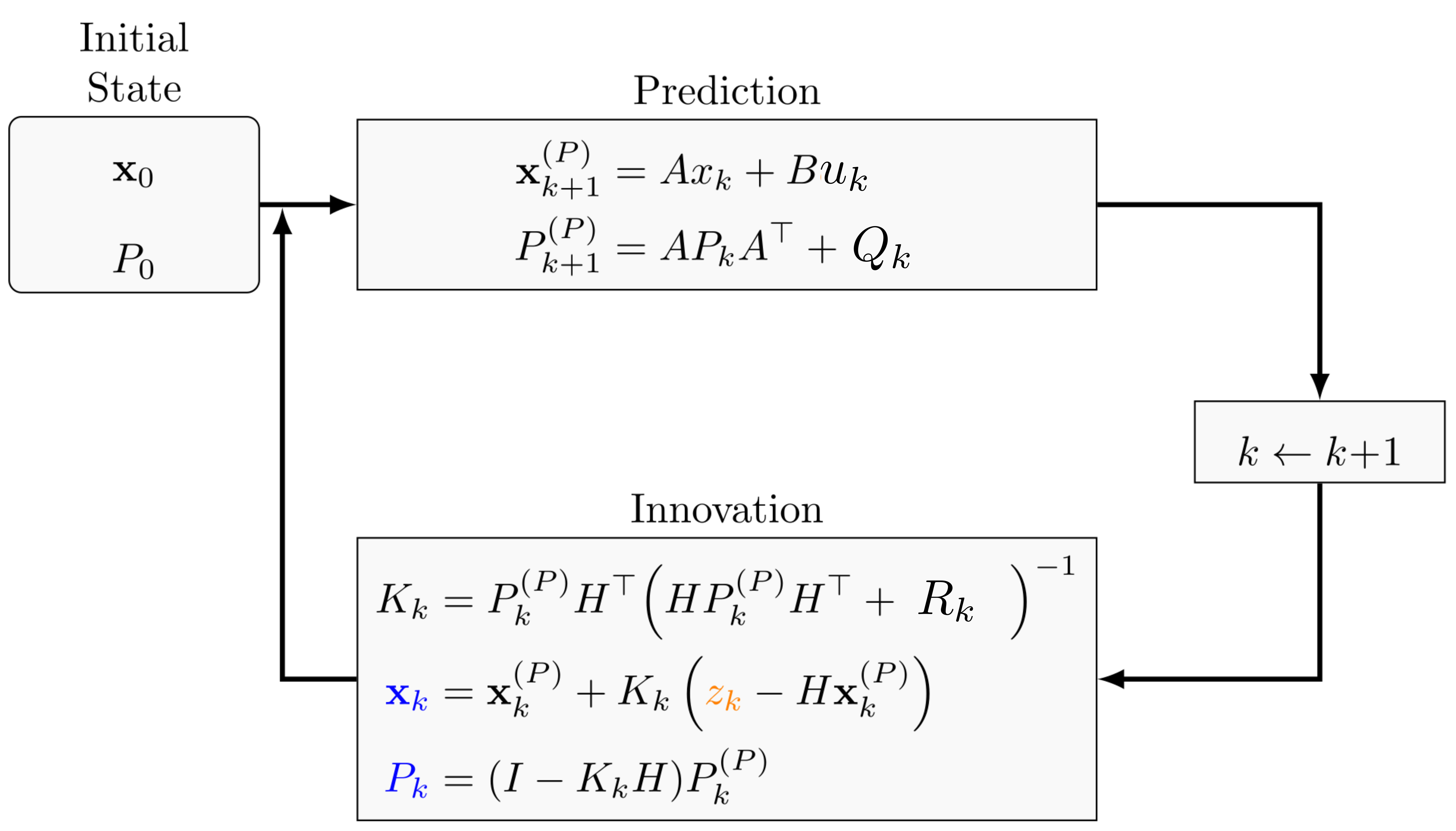
Modeling Assumptions
- System’s state evolution $\mathbf{x}_{k+1} = f(\mathbf{x}_k,u_k) + w_{\textit{x}}$ is linear and driven by
- Known input $u_k$
- Additive process noise $w_{\textit{x}}$ which is assumed to be a zero-mean, white and uncorrelated with known covariance matrix $Q(k)$
- The measurements $ z_k = h(x_k,u_k) + w_z $ are linear function of the state vector and the input vector with
- Additive zero-mean white noise with known covariance $R(k)$
- The initial state vector is a random variable with known mean $\mathbf{x}_0$ and covariance $P_0$ (initial uncertainty)
Under the above assumptions the Kalman Filter is the MMSE state estimator. If the random variables are not Gaussian, but one can still obtain their first two moments, then the KF is still the best linear MMSE estimator.
Why the standard KF is not enough
- Usually the motion models are nonlinear
- The measurement models are usually nonlinear
- Unable to capture mode changes(target maneuveres)
- Can’t handle cross-correlated noise
- Single target & unimodal method
Extended Kalman Filter
The EKF is a suboptimal state estimation algorithm for nonlinear systems.
Modeling Assumptions
- Same as the KF except that the state transition function $f$ and/or the measurement function $h$ are nonlinear, note that the noises are still assumed to enter additively into the state update/measurement equations.
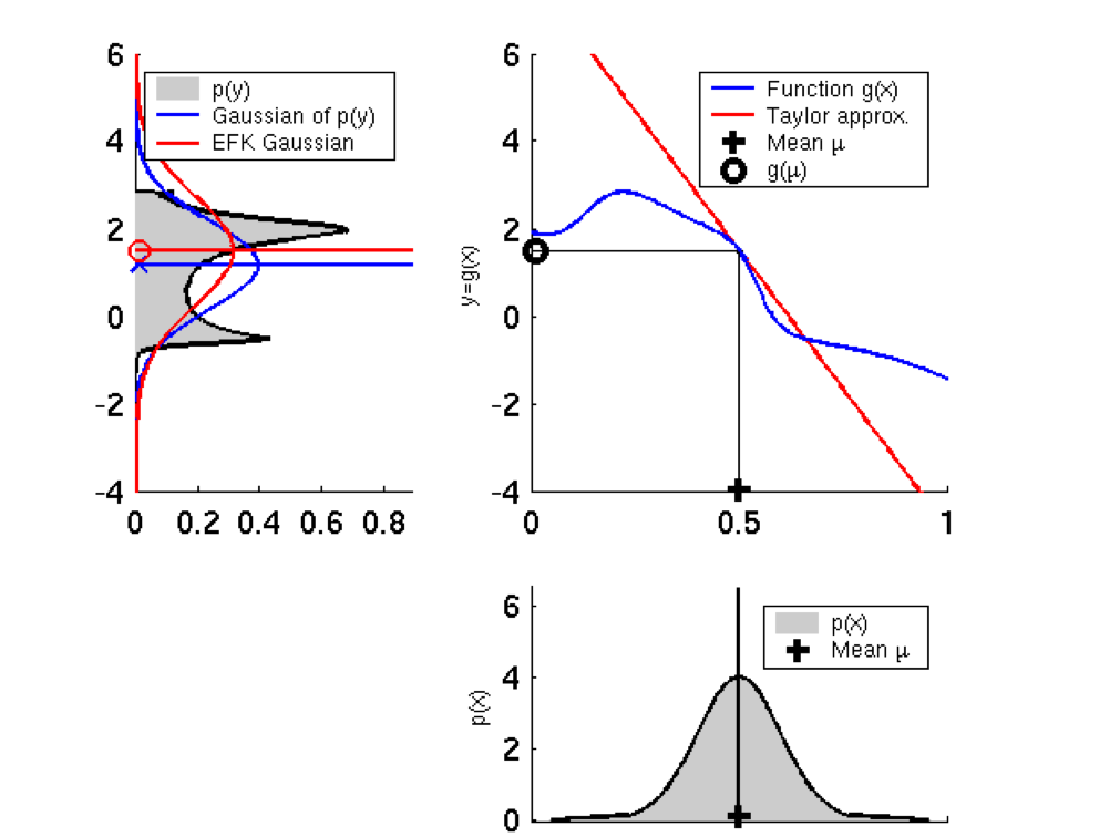
- First order Taylor expansion of the nonlinear functions around the current state is a reasonable approximation of the original nonlinear functions.
Taylor approximation of the CTRV motion models
A nonlinear motion model $x_{k} = f({x}{k-1})$ can be linearised around a known state $x{k-1}$
$$ f_{k-1} \approx F_{k-1} = \begin{bmatrix} \nabla_{x_{k-1}} f_{k-1}^{T}(x_{k-1}) \end{bmatrix}{x{k-1} \rightarrow\text{latest estimate}}^{T} $$
and for the CTRV motion model this leads to
$$ F_{{CTRV}_{k-1}} = \begin{bmatrix}1 &0 &\frac{sin(h+T\omega) - \sinh}{\omega} & \upsilon \frac{cos(h+T\omega)-cosh}{\omega} & \upsilon\frac{sinh -sin(h+T\omega) + T\omega cos(h+T\omega)}{\omega^{2}}\\ 0 &1 &-\frac{cos(h+T\omega) - cos(\omega)}{\omega} &\upsilon \frac{sin(h+T\omega)-sinh}{\omega} & \upsilon\frac{cos(h + T\omega) -cosh + T\omega sin(h+T\omega)}{\omega^{2}}\\ 0 &0 &1 &0 &0 \\ 0 &0 &0 &0 &1\end{bmatrix} $$
Taylor approximation of the measurement models
similarly, a measurement model $z_k=h(\mathbf{x_k})$ can be linearised around the latest motion propagated estimate $x_{k}$ as
$$ h_{k} \approx H_{k} = \begin{bmatrix} \nabla_{x_{k}} h_{k}^{T}(x_{k}) \end{bmatrix}{x{k} \rightarrow\text{motion updated estimate}}^{T} $$
For example, the radar model that measures distance and bearing to a target with known state vector $\mathbf{x}_k = [x,y,\upsilon,h,\omega]^T$, can be linearised as:
$$ H_k = \begin{bmatrix} \frac{x}{\sqrt{x^2+y^2}} &\frac{y}{\sqrt{x^2+y^2}} &0 &0 &0 \\ -\frac{y}{x^2+y^2} &\frac{x}{x^2+y^2} &0 &0 &0 \end{bmatrix} $$
Simulated EKF performance
- Motion model CTRV, sample time T = 100ms
- Measurement models, asynchronous measurements from:
- Noisy Radar measurements: bearing and distance, Ts=5 s
- Noisy Camera pixel measurements. The camera is measuring the targets horizontal target pixel location on the image plane every Ts=20s.
| Sample time | function | |
|---|---|---|
| Radar | 5s | n-linear |
| Camera | 20s | n-linear |
| CTRV Motion model | 0.1s | n-linear |
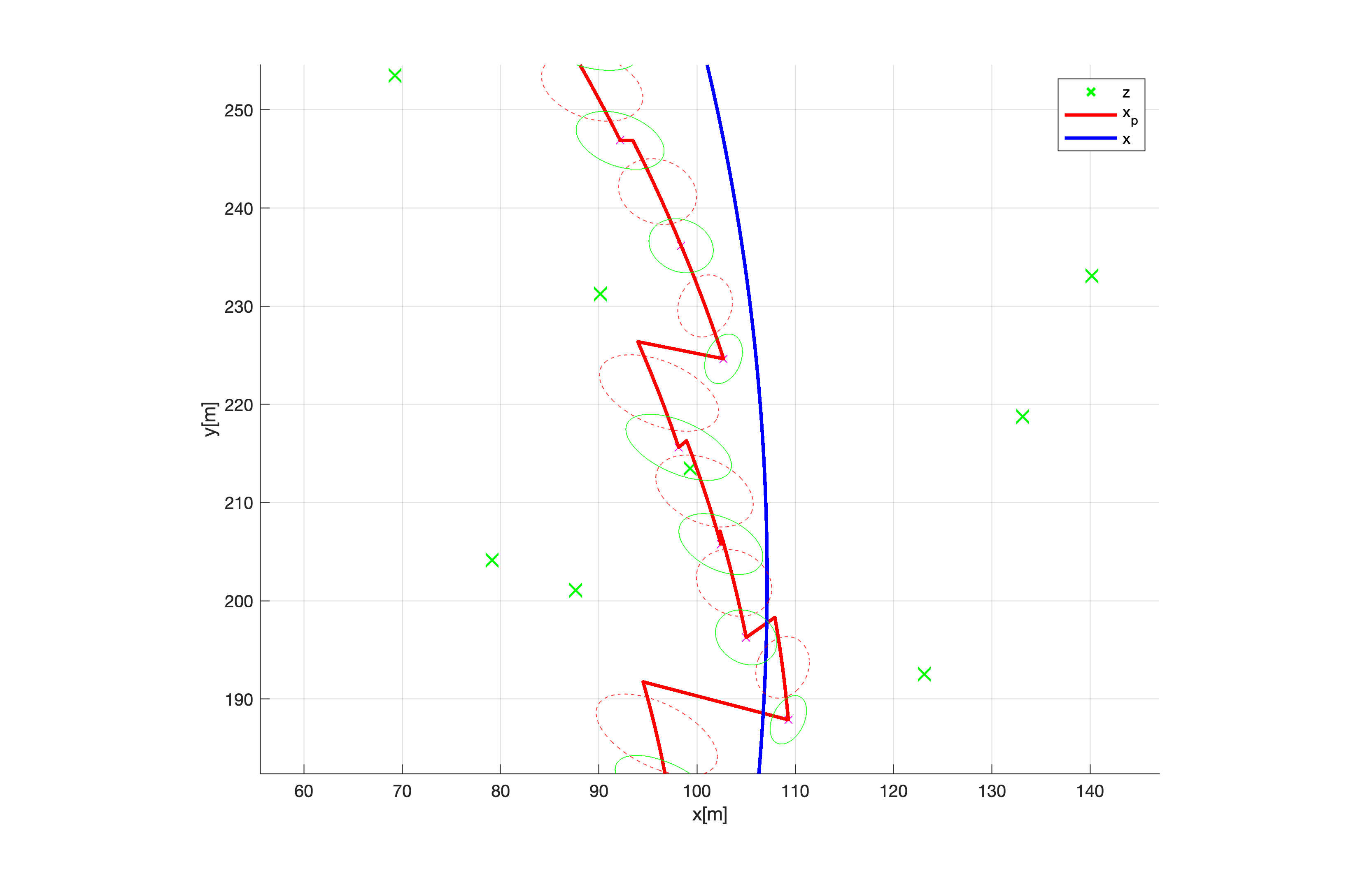
Having a close look at a segment of the trajectory one can observe the effect of using a CTRV model.
- Clearly the estimator is able to adapt to the step change in the turn rate but the convergence to the real track at the moment of the change is rather slow because the motion model that the filter is using assumes constant turn rate with low process noise.
- The red ellipses correspond to the estimated state uncertainty $P_k$ as propagated through the motion model.
- The green ellipses correspond to the estimated state uncertainty $P_k$ after incorporating a measurement $z_k$, whether that be a radar or a camera measurement.
| Illustration | Representation | Variable |
|---|---|---|
| Red ellipse | Predicted state-uncertainty $3\sigma$ area | $\hat{P}_k$ |
| Green ellipse | Corrected predicted state-uncertainty $3\sigma$ area | $\hat{P}_k$ |
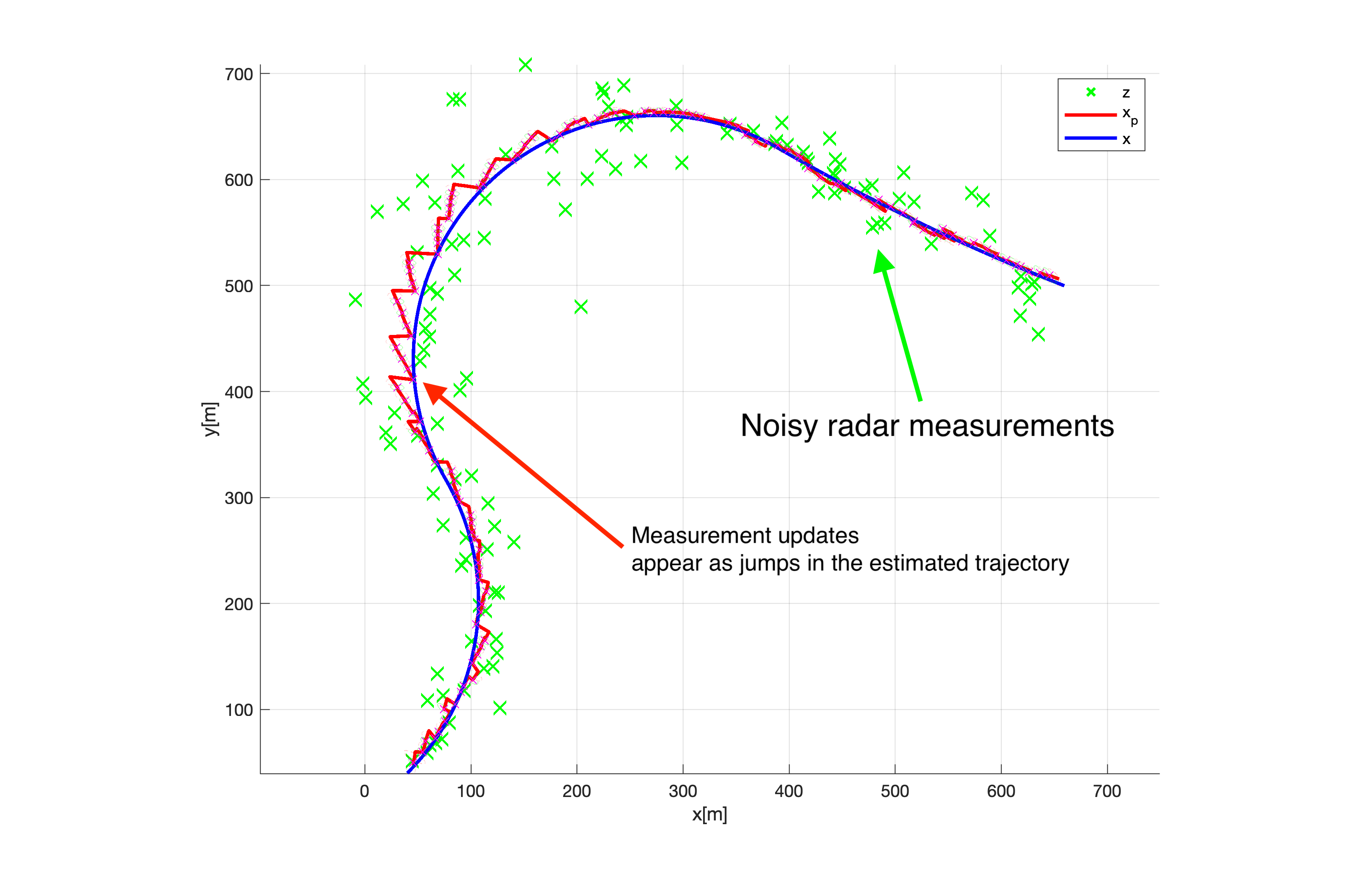
| Blue trajectory | Target’s real trajectory | $\mathbf{x}_{0:k}$ |
| Red trajectory | Estimated target’s state trajectory | $\hat{\mathbf{x}}_{0:k}$ |
| Green cross | Noisy radar measurements | $z_{radar}$ |
Filter performance
Performance graphs
The performance of the EKF single target tracker previously shown in 2D, is outlined in the following figures
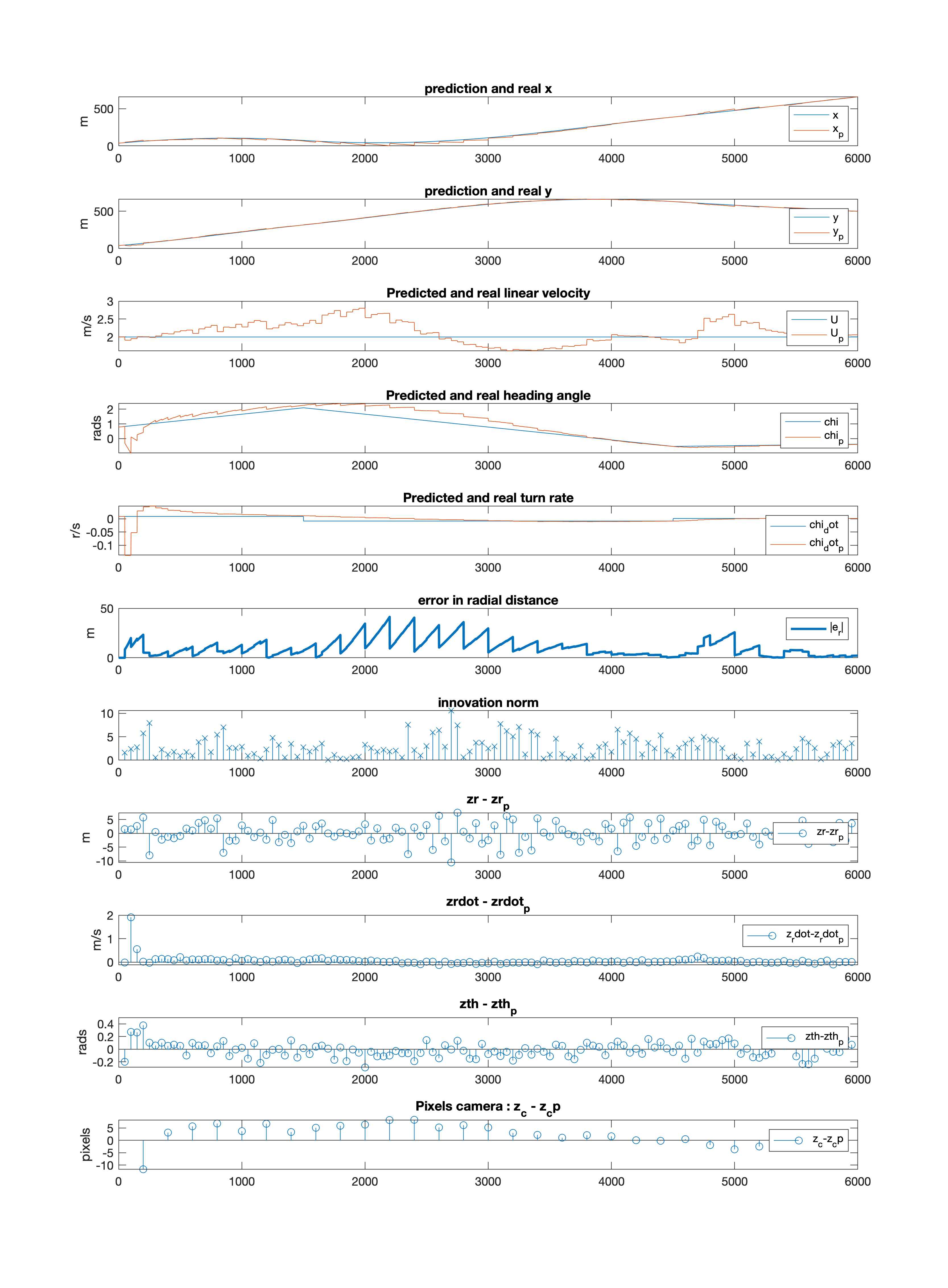
From top to bottom:
- Predicted target position $x_p$ and real target position $x$ w.r.t Seakeeping own-ship frame
- Predicted target position $y_p$ and real target position $y$ w.r.t Seakeeping own-ship frame
- Predicted target heading velocity $\upsilon_p$ and real target heading velocity $\upsilon$ w.r.t Seakeeping own-ship frame
- Predicted target heading velocity $h_p$ and real target heading velocity $h$ w.r.t Seakeeping own-ship frame
- Predicted target turn rate $\omega_{p}$ and real target turn rate $\omega$
- Absolute distance prediction error norm $|e| = \sqrt{(x-x_p)^2+(y-y_p)^2}$
- Innovation norm $|v|$, is a measure of how accurate the filter is tracking the real target, an unbound innovation norm implies that the observations do not match the predicted trajectory anymore i.e the tracker diverged.
- Innovation of the range measurements
- Innovation of the range rate Measurements
- Innovation of the bearing measurement
- Innovation of the camera localiser measurements
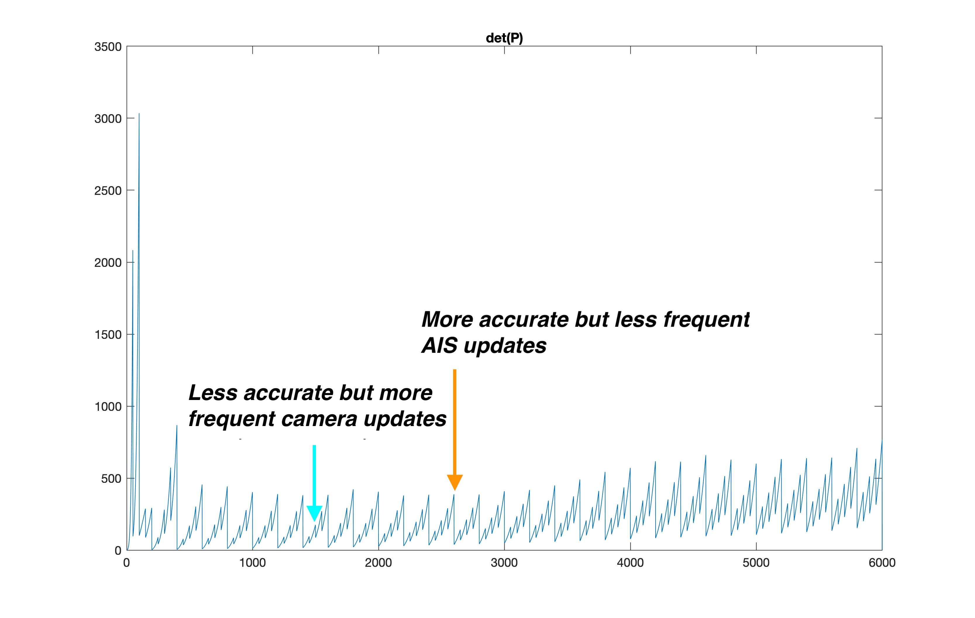
Determinant of $P_k$
Calculating the determinant $||P_k||$ of the first two columns and rows of the predicted state covariance matrix provides an indication of the magnitude of the tracking uncertainty of the target on the 2D tracking plane. Or in other words a measure of the surface of the plotted uncertainty ellipses. As seen in the figure below, measurement updates from different sensors are able to keep the uncertainty low.
Dimitrios Dagdilelis
ML/AI Engineer
Hey there, I enjoy making machines observe the world. If you have something interesting to share, there is no better time that now, connect with me and lets discuss.